Rational Bézier Curves and Circles in Rust

Introduction

There are important curves that cannot be represented precisely using Bézier curves. However, some of those curves, can be represented with rational Bézier curves.

While writing my crate on isogeometric analysis, I thought I could also try to implement rational Bézier curves and use that implementation to draw perfect circles. I noticed not many documents are available about this topic, but some^[1][2] were pretty helpful.

Rational Bézier Curves

A n-th degree rational Bézier curve is defined as:

$$\boldsymbol{C}(\xi)=\frac{\sum\limits_{i=0}^{n}B_{i}^{n}(\xi)w_{i}\boldsymbol{P}_{i}}{\sum\limits_{i=0}^{n}B_{i}^{n}(\xi)w_{i}}$$

or with homogeneous coordinates:

$$\boldsymbol{C}^{w}(\xi)=\sum_{i=0}^{n}B_{i}^{n}(\xi)\boldsymbol{P}_{i}^{w}$$

where $\boldsymbol{P}_i^w$ are the weighted control points.

Rational Bézier Curve for the Circle

To find the proper rational Bézier curve to precisely draw the circle, I started from the assumption that a rational Bézier could actually draw a perfect circular arc (I wasn’t completely sure at first).

I considered the following construction, where $r$ is the radius of the circle:

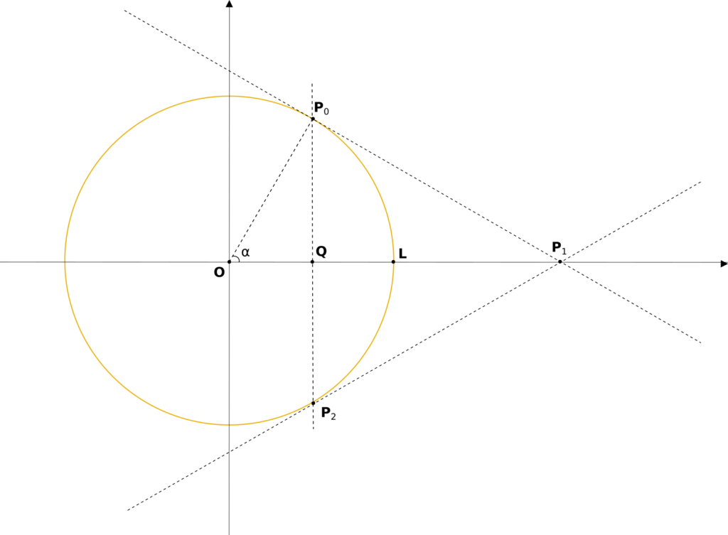
The arc from $\boldsymbol{P}_0$ to $\boldsymbol{P}_2$ is the one I’d like to build. If a rational Bézier like the one I’m trying to build actually existed, I’d need to determine the three weights to define it. The line passing by $\boldsymbol{P}_0$ and $\boldsymbol{P}_1$ and the line passing by $\boldsymbol{P}_1$ and $\boldsymbol{P}_2$ are tangent to the circle by construction. As a Bézier curve is always tangent to the first and the last leg, I assume $w_0$ and $w_2$ should be equal to 1. I still need $w_1$, but I can state that my rational Bézier curve must pass by $\boldsymbol{L}$, and, by symmetry, I’d say it should do so in $\frac{1}{2}$:

$$\boldsymbol{L}=\boldsymbol{C}\left(\frac{1}{2}\right)=\left[\begin{array}{c} r\\ 0 \end{array}\right]=\frac{\sum\limits_{i=0}^{2}B_{i}^{2}\left(\frac{1}{2}\right)\cdot w_{i}\boldsymbol{P}_{i}}{\sum\limits_{i=0}^{2}B_{i}^{2}\left(\frac{1}{2}\right)\cdot w_{i}}$$

I can now replace what I already know by construction:

$$\displaylines{w_{0}=1,w_{2}=1,\boldsymbol{P}_{0}=\left[\begin{array}{c}
r\cdot cos(\alpha)\\
r\cdot sin(\alpha)
\end{array}\right],\\
\boldsymbol{P}_{1}=\left[\begin{array}{c} \frac{r}{cos(\alpha)}\\ 0 \end{array}\right],\boldsymbol{P}_{2}=\left[\begin{array}{c}
r\cdot cos(\alpha)\\
-r\cdot sin(\alpha)
\end{array}\right].}$$

resulting in:

$$\left[\begin{array}{c}
r\\
0
\end{array}\right]=\frac{B_{0}^{2}\left(\frac{1}{2}\right)\left[\begin{array}{c}
r\cdot cos(\alpha)\\
r\cdot sin(\alpha)
\end{array}\right]+B_{1}^{2}\left(\frac{1}{2}\right)\left[\begin{array}{c}
\frac{r}{cos(\alpha)}\\
0
\end{array}\right]+B_{2}^{2}\left(\frac{1}{2}\right)\left[\begin{array}{c}
r\cdot cos(\alpha)\\
-r\cdot sin(\alpha)
\end{array}\right]}{B_{0}^{2}\left(\frac{1}{2}\right)+B_{0}^{1}\left(\frac{1}{2}\right)\cdot w_{1}+B_{2}^{2}\left(\frac{1}{2}\right)}$$

The coordinates of $\boldsymbol{P}_1$ can be determined by looking at the right triangle $\boldsymbol{O}\boldsymbol{P}_0\boldsymbol{P}_1$. By computing Bernstein polynomials:

$$\left[\begin{array}{c}
r\\
0
\end{array}\right]=\frac{1}{1+w_{1}}\cdot\left[\begin{array}{c}
r\cdot cos\left(\alpha\right)+\frac{w_{1}\cdot r}{cos\left(\alpha\right)}\\
0
\end{array}\right]$$

which means:

$$r=\frac{r}{1+w_{1}}\cdot\left(cos(\alpha)+\frac{w_{1}}{cos(\alpha)}\right)$$

and therefore:

$$w_1=cos(\alpha)$$

This means that my circular arc, with the assumption I made above, can be drawn for any radius $r > 0$ by using $w_1$ as found above. Another relevant assumption is that $\alpha\in\left(0,90\right)$. By simply rotating the circular arc I can draw the rest of the circle.

Correctness

By itself, this procedure does not prove that the curve resulting from this data is a perfect circular arc. It only proves that the curve will pass by points $\boldsymbol{P}_0$, $\boldsymbol{P}_2$ and $\boldsymbol{L}$. We can however prove that the result is a circular arc by verifying the identity:

$$d\left(\boldsymbol{O},\boldsymbol{C}\left(\xi\right)\right)=r,\forall\xi\in\left[0,1\right]$$

to simplify, I considered $\boldsymbol{O}=\left[\begin{array}{c}
0\\
0
\end{array}\right]$, so I got to:

$$\sqrt{C_{x}\left(\xi\right)^{2}+C_{y}\left(\xi\right)^{2}}=r,\forall\xi\in\left[0,1\right]$$

By entering data in Maxima I got:

$$\sqrt{\frac{{{\left( \sin{(\alpha)} r {{\left( 1-\xi\right) }^{2}}-\sin{(\alpha)} r {{\xi}^{2}}\right) }^{2}}}{{{\left( {{\xi}^{2}}+2 \cos{(\alpha)} \left( 1-\xi\right) \xi+{{\left( 1-\xi\right) }^{2}}\right) }^{2}}}+\frac{{{\left( \cos{(\alpha)} r {{\xi}^{2}}+2 r\, \left( 1-\xi\right) \xi+\cos{(\alpha)} r {{\left( 1-\xi\right) }^{2}}\right) }^{2}}}{{{\left( {{\xi}^{2}}+2 \cos{(\alpha)} \left( 1-\xi\right) \xi+{{\left( 1-\xi\right) }^{2}}\right) }^{2}}}}$$

by using the fundamental theorem of the trigonometry Maxima returns $|r|$. This means that the resulting rational Bézier curve is, in fact, a circular arc.

Building the Bézier Curve

Summing up, given is a radius $r$ and a number $n$ of patches we want to use, the crate:

• computes $\alpha=\frac{\pi}{n}$;
• computes even control points as:

$$\boldsymbol{P}_{2i}=\left[\begin{array}{c}
r\cdot sin\left(2\cdot i\cdot \alpha\right)\\
-r\cdot cos\left(2\cdot i\cdot \alpha\right)\end{array}\right],i=0,..,n$$

• computes odd control points as:

$$\boldsymbol{P}_{2i+1}=\left[\begin{array}{c}
\frac{r}{cos\left(\alpha\right)}\cdot sin\left(\left(2\cdot i + 1 \right)\cdot \alpha\right)\\
-\frac{r}{cos\left(\alpha\right)}\cdot cos\left(\left(2\cdot i + 1 \right)\cdot \alpha\right)\end{array}\right],i=0,..,n-1$$

• computes weigths as:

$$w_{2n}=1,i=0,..,n$$

$$w_{2n+1}=cos\left(\alpha\right),i=0,..,n-1$$

This results in a set of quadratic rational Bézier curves. By drawing all these curves, you should get the circle. This is what one of the unit tests does:

let circle = BezierCircle {
    radius: r,
    segments: s
};
let ratbezs = circle.compute().unwrap();
for ratbez in ratbezs.iter() {
    let mut computed = RealPoint2d::origin();
    for i in 0..=1000 {
        let input = RealPoint1d::point1d((i as f64)/1000.);
        ratbez.evaluate_fill(&input, &mut computed);
        let dist = RealPoint2d::origin().dist(&computed);
        assert_approx_eq!(f64, dist, r as f64, epsilon = 1E-6);
    }
}

it creates a circle of radius $r$ with $s$ curves. The class BezierCircle executes the steps above and returns a sequence of quadratic rational Bézier curves. The unit test then evaluate each of these curves and confirms that the distance between the computed point and the origin is exactly $r$.

You can find all the code in the repo: https://github.com/carlonluca/isogeometric-analysis.

Bye! 😉

[1]: https://pages.mtu.edu/~shene/COURSES/cs3621/NOTES/spline/NURBS/RB-circles.html
[2]: https://ctan.math.illinois.edu/macros/latex/contrib/lapdf/rcircle.pdf